Look at your data!

Once again, we will start by looking at our data! Let’s see if there is any evidence for richness varying with catchment type. We can do this with the plot function, which acts similarly to boxplot when we are plotting continuous data against factors.

plot(Richness ~ Type, data=Inverts)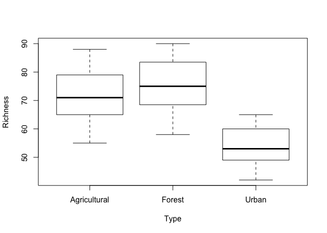

It looks like invertebrate species richness is fairly comparable between streams in agricultural and forested areas, but lower in urban areas. However, there is enough variation that we don’t know if this will be a statistically significant difference. So let’s run an ANOVA and find out.

Fit the model

To fit an ANOVA to the data, we can use either lm or aov, which will effectively do the same thing. The main difference is how the output is presented in a call to summary. Let’s use aov, which will put the output of summary in a form that makes sense for ANOVA results.

The help file for aov (?aov) notes that the default contrasts in R are not orthogonal, and aov will work better with orthogonal contrasts, so let’s start by setting them. Contrasts have to do with how the levels of each factor are compared to each other in a linear model. Information on the various contrasts available in R can be found in the help file for specific contrasts (e.g., ?contr.helmert), and more detail on how each contrast setting works can be found in this post on unordered contrats and a UCLA Stat Consulting Group page.

The following code both sets the contrasts to be orthogonal (contr.helmert for unordered factors and contr.poly for ordered factors) and assigns the original options to op so that they can be re-set using options(op). (You can also set the contrasts within the call to lm or aov later on, using the argument contrasts, but instead we will do it at the beginning for convenience - it will now apply to all downstream models.)

# Set default values to op to be able to re-set later; 
# set current values to contr.helmert for unordered factors and contr.poly for ordered factors.
op <- options(contrasts = c(unordered="contr.helmert", ordered="contr.poly")) 

# Check contrasts in current settings, if you'd like
options()$contrasts

##       unordered         ordered 
## "contr.helmert"    "contr.poly"

Now we can fit the model. We’ll store it as a named object so that we can work with it more easily later.

You can name this object however you want, but it’s good to be consistent with your naming scheme throughout your code, so that you can easily identify what kind of object you are working with. There are multiple naming conventions used in R and R packages, as well as multiple style guides (e.g., see here). In the case below, the . in the model name is only for convenient reading. (There is some debate on when and how this . should be used. This is in part because the . has a specific meaning in other programming languages, whereas it is simply another character in an R variable name.)

InvertsType_mod <- aov(Richness ~ Type, data=Inverts)

Now let’s take a look at the model object with summary.

summary(InvertsType_mod)

##             Df Sum Sq Mean Sq F value   Pr(>F)    
## Type         2   2094  1046.8   11.23 0.000483 ***
## Residuals   21   1958    93.3                     
## ---
## Signif. codes:  0 '***' 0.001 '**' 0.01 '*' 0.05 '.' 0.1 ' ' 1

This output gives us the results of an F-test with the null hypothesis that the groups are from the same statistical population, which would mean that their means do not vary. We can see that p<0.001, indicating that the groups are likely from different populations. Thus, species richness significantly varies with catchment type.

NOTE: The ANOVA table given by summary with an aov model gives results using Type I SS (Sum of Squares). The function anova gives the same output as summary, and similarly uses Type I SS. This does not matter for a one-way ANOVA, but it absolutely does with multiple factors! We will cover this further in the Two-way ANOVA section. For now, the point to remember is that you should not accidentally report your results from summary on an ANOVA model unless you are doing a one-way ANOVA, or if your experimental question is such that Type I SS makes sense (which is not common).

Check model assumptions

Of course, we can’t use this model unless we know that we have satisfied the model’s assumptions! As with linear regression, we need to check the homogeneity and normality of the residuals. We will make the plots as before, starting with a histogram and a QQ plot of the residuals, and then comparing the residuals to the explanatory variable, Type.

par(mfrow=c(2,2))  # Set plot layout
hist(resid(InvertsType_mod), las=1)  # Look at distribution of residuals
qqnorm(resid(InvertsType_mod), las=1)  # Compare distribution of residuals to a normal distribution
qqline(resid(InvertsType_mod))
plot(fitted(InvertsType_mod), resid(InvertsType_mod), las=1)  # Do residuals vary by fitted values?
plot(Inverts$Type, resid(InvertsType_mod), las=1)  # Do the residuals vary by group?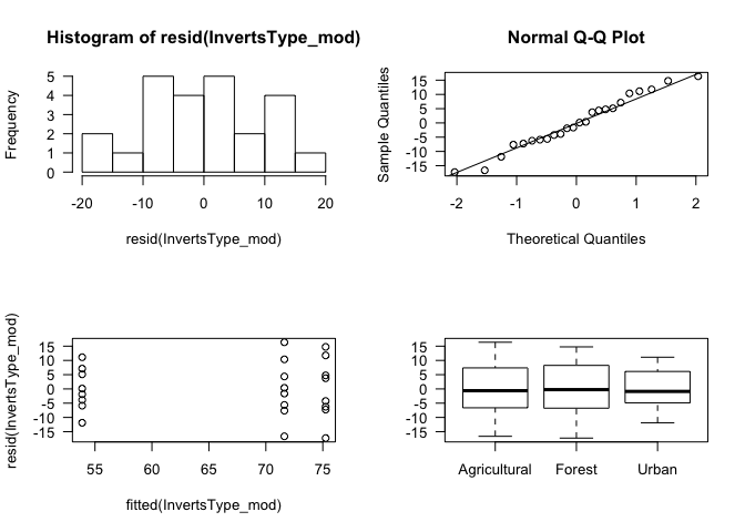

par(mfrow=c(1,1))  # Re-set plot layout

These plots give us good news. The distribution of residuals doesn’t look extraordinarily normal in the histogram, but this could be an effect of small sample size, and the QQ plot suggests a mostly normal distribution with a few potentially outlying points. The bottom plots suggests that the residuals are comparable among groups (homogeneity). On the plot of the residuals versus the fitted values, the values on the x-axis might seem obscure at first - these are the means for the three groups (Agricultural, Forest, and Urban).

We can also make similar plots by making a function call to plot using the model as input. In this case, the function will automatically point out potential outliers.

par(mfrow=c(2,2))  # Set plot layout for 4 plots
plot(InvertsType_mod, las=1)  # Plot residuals for our ANOVA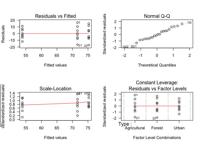

par(mfrow=c(1,1))  # Re-set plot layout

Now we can see that there are three points that are potential outliers. If these were real data, it could be useful to examine these specific points further to determine whether there is any reason not to include them in the analysis.

These plots indicate that out model is appropriate for these data, and we can report the results. Note, however, that the opposite result - e.g., discovering that the residuals are not normally distributed - can still be immensely useful, as visualizing the residuals (and their distribution) can help you determine what would be an appropriate approach. For example, if you saw that your residuals were right-skewed, this would suggest that log-transformation of the dependent variable (before fitting the ANOVA) would result in normally distributed residuals.

Post-hoc testing

We’ve interpreted the results to mean that species richness varies with catchment type. But, which catchment types differ from each other? To assess this, we can use a Tukey test with the function TukeyHSD (for Tukey’s “Honestly Significant Difference” method).

TukeyHSD(InvertsType_mod)

##   Tukey multiple comparisons of means
##     95% family-wise confidence level
## 
## Fit: aov(formula = Richness ~ Type, data = Inverts)
## 
## $Type
##                        diff        lwr       upr     p adj
## Forest-Agricultural   3.625  -8.545074 15.795074 0.7364753
## Urban-Agricultural  -17.750 -29.920074 -5.579926 0.0038490
## Urban-Forest        -21.375 -33.545074 -9.204926 0.0006580

The top part of the output tells us that we’re using 95% confidence intervals. If for some reason we wanted to change this, we could use the argument conf.level, which defaults to 0.95.

The table below $Type gives us the p-values for comparisons between groups. From this, we can see that at a significance level of 0.05 (\(\alpha\) = 0.05), species richness in forested and agricultural areas are comparable, whereas that of urban areas differs significantly from the two other groups.

Look at your data (again)!

We will of course start by looking at the data. We can look at species richness by country, to complement the above plot of species richness by catchment type, or we can look at species richness by all country-type groups, using boxplot.

p <- par(mar=c(10,4,2,2))  # Save current parameters & re-set margins to allow for long x-axis labels
boxplot(Richness ~ Type + Country, data=Inverts, las=2)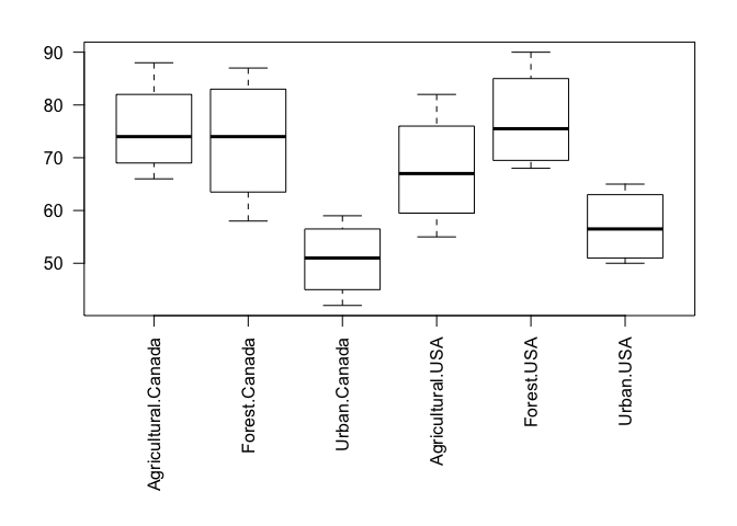

par(p)  # Reset margins

We can still see the differences between catchment type, but it’s difficult to tell whether there are differences by country, especially between urban catchments. So, let’s add Country to our model to see if it has an effect.

Fit the model

Implementing a two-way ANOVA is similar to implementing ANOVA, in that we will use the model function (aov). It is also similar to multiple regression, in terms of the way that we specify multiple factors or explanatory variables. Here, we will use * to include both main effects and their interaction.

Inverts2way_mod <- aov(Richness ~ Type * Country, data=Inverts)
summary(Inverts2way_mod)  # F-test with Type I Sum of Squares (probably not appropriate!)

##              Df Sum Sq Mean Sq F value  Pr(>F)    
## Type          2 2093.6  1046.8  10.904 0.00079 ***
## Country       1    4.2     4.2   0.043 0.83731    
## Type:Country  2  226.1   113.0   1.178 0.33068    
## Residuals    18 1728.0    96.0                    
## ---
## Signif. codes:  0 '***' 0.001 '**' 0.01 '*' 0.05 '.' 0.1 ' ' 1

Here is where it is important to remember that summary gives you results using Type I Sum of Squares! So, do not stop here to determine the significance of the independent variables.

# With drop1, the scope argument designates the terms to be dropped; the . means all of them.
drop1(Inverts2way_mod, scope = ~., test="F")  

## Single term deletions
## 
## Model:
## Richness ~ Type * Country
##              Df Sum of Sq    RSS    AIC F value    Pr(>F)    
## <none>                    1728.0 114.64                      
## Type          2   2093.58 3821.6 129.69 10.9041 0.0007901 ***
## Country       1      4.17 1732.2 112.70  0.0434 0.8373079    
## Type:Country  2    226.08 1954.1 113.59  1.1775 0.3306785    
## ---
## Signif. codes:  0 '***' 0.001 '**' 0.01 '*' 0.05 '.' 0.1 ' ' 1

library("car")

## 
## Attaching package: 'car'

## The following object is masked from 'package:dplyr':
## 
##     recode

Anova(Inverts2way_mod, type="III")  # Specify Type III SS

## Anova Table (Type III tests)
## 
## Response: Richness
##              Sum Sq Df   F value    Pr(>F)    
## (Intercept)  107468  1 1119.4601 < 2.2e-16 ***
## Type           2094  2   10.9041 0.0007901 ***
## Country           4  1    0.0434 0.8373079    
## Type:Country    226  2    1.1775 0.3306785    
## Residuals      1728 18                        
## ---
## Signif. codes:  0 '***' 0.001 '**' 0.01 '*' 0.05 '.' 0.1 ' ' 1

Check assumptions

To use this model, we need to check that its assumptions have been met. We will look at the model residuals as before.

par(mfrow=c(2,2))  # Set plot layout
plot(Inverts2way_mod, las=1)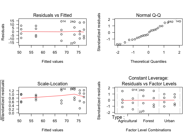

par(mfrow=c(1,1))  # Re-set plot layout

And as before, our residuals look fairly normal and homogeneous, so we can report the model output.

Post-hoc testing

We may still wonder about the differences between levels of the significant factor, Type. With a 2-way ANOVA, we can apply a Tukey test using the function lsmeans in the package lsmeans, along with the function cld, which controls the output that is displayed. The first argument to cld is an object created by lsmeans. lsmeans requires us to specify the model as well as the variable to test (e.g., Type), and give us confidence intervals as output, which we could use to determine which groups differ. We can also use cld to figure this out for us. For cld, we can to specify the p-value as alpha, the post-hoc test to use as adjust, and whether to use letters instead of the default to numbers for comparing groups.

If you have not already done so, be sure to install lsmeans and associated dependencies, i.e. with install.packages("lsmeans", dependencies = TRUE).

library("lsmeans")

## Loading required package: estimability

# Which Types vary from the others, using a Tukey test?
    cld(lsmeans(Inverts2way_mod, specs="Type"), alpha=0.05, adjust="tukey", Letters=letters) 

## NOTE: Results may be misleading due to involvement in interactions

##  Type         lsmean       SE df lower.CL upper.CL .group
##  Urban        53.875 3.464102 18 44.76064 62.98936  a    
##  Agricultural 71.625 3.464102 18 62.51064 80.73936   b   
##  Forest       75.250 3.464102 18 66.13564 84.36436   b   
## 
## Results are averaged over the levels of: Country 
## Confidence level used: 0.95 
## Conf-level adjustment: sidak method for 3 estimates 
## P value adjustment: tukey method for comparing a family of 3 estimates 
## significance level used: alpha = 0.05

Take a look at the output under .group. Here we can see that the Urban streams have significantly different invertebrate species richness than the other catchment types. And, this approach gives us the added convenience of letters that can be used to denote significance on a figure!

If the interaction were significant and we wanted to do pairwise comparisons between groups, we could use the lsmeans function with specs = pairwise ~ Type * Country. You can try this out if you’re curious about the output.

So it looks like we can conclude that (in the world represented by this fake data) species richness varies among catchment types, with lower richness in urban areas - but we can only conclude this if the model assumptions are met!