Joining data frames with dplyr
Why, and what?
Sometimes you may want to conduct analyses with data that are in separate data frames, and you need to combine the data frames into one to do so. This often happens when you run multiple analyses on the same set of samples. Alternatively, you might want to compare data frames to determine which samples are in both, or which samples are missing from one.
Using functions to accomplish this is much more efficient than trying to match entries manually!
There are multiple ways to join two data frames, depending on the variables and information we want to include in the resulting data frame. The package dplyr has several functions for joining data, and these functions fall into two categories, mutating joins and filtering joins.
- Mutating joins add new variables from one table to matching observations in another table.
- Filtering joins retain observations in one table based on whether or not they match the observations in another table.
In class today, we will talk about two types of mutating joins: left joins and full joins. However, for your reference, all joins from both categories are demonstrated below. For more information and examples, see the dplyr Two-table verbs vignette.
Mutating joins
There are four types of mutating joins, which we will explore below:
- Left joins (
left_join) - Right joins (
right_join) - Inner joins (
inner_join) - Full joins (
full_join)
Mutating joins add variables to data frame x from data frame y based on matching observations between tables. The different joins have different controls on, or rules for, which observations to include.
Let’s start with the hypothetical data frame described in the reshaping lesson, containing nutrient concentrations for 3 replicates for each of 2 treatments. We also have measurements of extractable organic carbon from the same samples, except that replicate 2 of treatment 1 was lost, and the carbon data file contains data for another treatment, treatment 3.
We’ll read in the data from .csv files.
nutrients <- read.csv(file="Data/Experiment_nutrients.csv")
nutrients
## Treatment Replicate Ammonium Nitrate Nitrite
## 1 1 1 8.2 1.7 0.4
## 2 1 2 6.9 3.6 1.5
## 3 1 3 12.1 2.8 0.8
## 4 2 1 10.5 0.4 0.7
## 5 2 2 8.6 2.7 1.2
## 6 2 3 7.8 4.1 0.9carbon <- read.csv(file="Data/Experiment_carbon.csv")
carbon## Treatment Replicate Carbon
## 1 1 1 42.5
## 2 1 3 49.1
## 3 2 1 40.8
## 4 2 2 50.4
## 5 2 3 50.8
## 6 3 1 45.6
## 7 3 2 48.7
## 8 3 3 43.5Left join
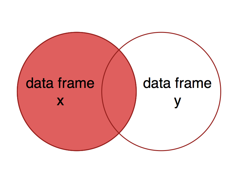
Let’s say that we want to add data on carbon concentration to the observations in the nutrients data frame. Specifically, we want to keep all of the observations in the nutrients data frame, and add another variable from the carbon data frame, Carbon, that contains carbon data when present and NA when values are missing. To do this, we can use the function left_join. This the type of join that you will likely want to use most often.
The term left join can be explained using a Venn diagram. The circle on the left is data frame x, and the one on the right is data frame y. The overlap between the two circles represents the observations with keys that are present in both data frames. The result of a left join is all of data frame x, plus the parts of data frame y with overlapping keys - i.e., the left side of the Venn diagram.
To do a left join on nutrients, adding variables from carbon, we would use the following syntax.
nutrients %>%
  left_join(y=carbon, by=c("Treatment","Replicate"))
## Treatment Replicate Ammonium Nitrate Nitrite Carbon
## 1 1 1 8.2 1.7 0.4 42.5
## 2 1 2 6.9 3.6 1.5 NA
## 3 1 3 12.1 2.8 0.8 49.1
## 4 2 1 10.5 0.4 0.7 40.8
## 5 2 2 8.6 2.7 1.2 50.4
## 6 2 3 7.8 4.1 0.9 50.8The argument y specifies the data frame from which to find data to add to nutrients. You can specify x as the data frame to act on, which would be nutrients, but we have passed it via %>% instead. The last argument, by, specifies which columns to join by - i.e., the keys. The default is to do a natural join, which means that the function will use all columns that are present in both data frames.
Let’s explore the by argument a bit further. What happens if we do a left join using only one of the by variables specified above, e.g., Treatment? What has happened to give the results below?
nutrients %>%
  left_join(y=carbon, by=c("Treatment"))
## Treatment Replicate.x Ammonium Nitrate Nitrite Replicate.y Carbon
## 1 1 1 8.2 1.7 0.4 1 42.5
## 2 1 1 8.2 1.7 0.4 3 49.1
## 3 1 2 6.9 3.6 1.5 1 42.5
## 4 1 2 6.9 3.6 1.5 3 49.1
## 5 1 3 12.1 2.8 0.8 1 42.5
## 6 1 3 12.1 2.8 0.8 3 49.1
## 7 2 1 10.5 0.4 0.7 1 40.8
## 8 2 1 10.5 0.4 0.7 2 50.4
## 9 2 1 10.5 0.4 0.7 3 50.8
## 10 2 2 8.6 2.7 1.2 1 40.8
## 11 2 2 8.6 2.7 1.2 2 50.4
## 12 2 2 8.6 2.7 1.2 3 50.8
## 13 2 3 7.8 4.1 0.9 1 40.8
## 14 2 3 7.8 4.1 0.9 2 50.4
## 15 2 3 7.8 4.1 0.9 3 50.8Take a look at Replicate.x and Replicate.y to sort out what has happened here. The variable Replicate was present in both data frames, and the new data frame includes a variable for each, specified by “.x” or “.y” at the end of the variable name. Also, the number of observations has increased. Remember that we tried to join by Treatment. The problem here is that there are multiple observations (Replicates) for each Treatment value in both x and y, so the resulting data frame includes all combinations of Replicate.x and Replicate.y within each Treatment.
Note that this may not be what you wanted, but it does not result in an error or warning! This is a good demonstration of why it’s important to understand the behaviour of functions that you use, and to check the results of intermediate steps in your analysis.
Challenge
Write out the code specifying the above left join (adding
carbondata tonutrientsdata) with and without a pipe (%>%).What happens if you use a left join to add
nutrientsdata to thecarbondata set, rather than vice versa?The data frame
climateshas information on mean annual temperature and precipitation for the sites in thetreesdata frame. Read inclimates.csv(andtrees.csvif you have not already done so), and use aleft_jointo add these climate data totrees. Take a look at the data first to determine which variable(s) to join by.Read in two files,
genes.csvandmetals.csv, and call the resulting data framesgenesandmetals.geneshas data on the abundance of different nitrogen cycling genes in soils at several agricultural sites, andmetalshas data on concentrations of different metals in soils at some of the same agricultural sites. Use a left join to add the metal concentration data to the observations ingenes. Why do you get a warning message? (Hint: Think back to the lesson on factors!)
Right join
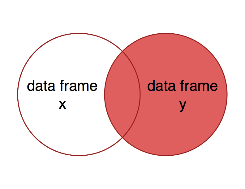
A right join is conceptually similar to a left join, but includes all the observations of data frame y and matching observations in data frame x - the right side of the Venn diagram.
What would you expect to get as a result of a right join using x = nutrients and y = carbon?
nutrients %>%
  right_join(y=carbon, by=c("Treatment", "Replicate"))
## Treatment Replicate Ammonium Nitrate Nitrite Carbon
## 1 1 1 8.2 1.7 0.4 42.5
## 2 1 3 12.1 2.8 0.8 49.1
## 3 2 1 10.5 0.4 0.7 40.8
## 4 2 2 8.6 2.7 1.2 50.4
## 5 2 3 7.8 4.1 0.9 50.8
## 6 3 1 NA NA NA 45.6
## 7 3 2 NA NA NA 48.7
## 8 3 3 NA NA NA 43.5Challenge
- How does the result from
right_join(x=nutrients, y=carbon)compare to that ofleft_join(x=carbon, y=nutrients)?
Inner join
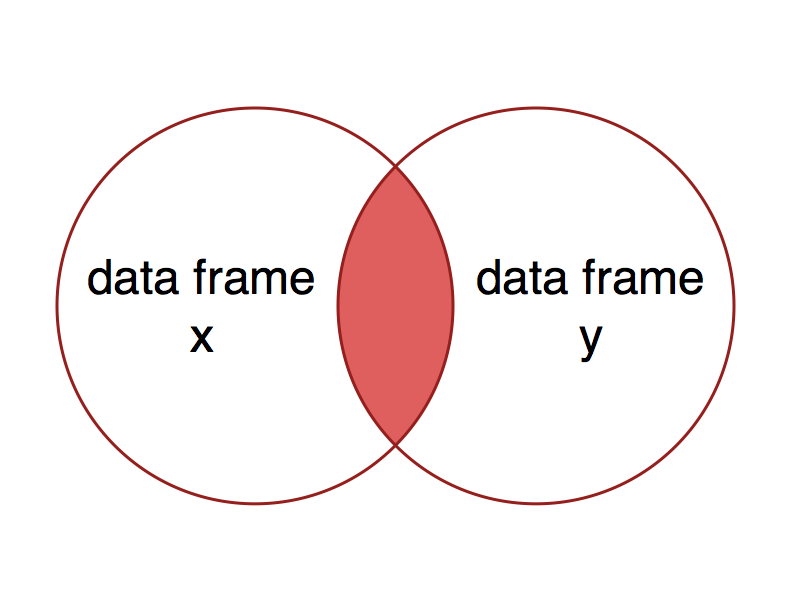
What if you want to include only the observations in both data frames, and omit observations with missing data? In this case, you can use an inner join.
An inner join includes observations with keys that are present in both data frames. This is the same as keeping only the observations in x that have a matching observation in y.
What would you expect to get as a result of an inner join using x = nutrients and y = carbon?
nutrients %>%
  inner_join(y=carbon, by=c("Treatment", "Replicate"))
## Treatment Replicate Ammonium Nitrate Nitrite Carbon
## 1 1 1 8.2 1.7 0.4 42.5
## 2 1 3 12.1 2.8 0.8 49.1
## 3 2 1 10.5 0.4 0.7 40.8
## 4 2 2 8.6 2.7 1.2 50.4
## 5 2 3 7.8 4.1 0.9 50.8You can see that Replicate 2 of Treatment 1 is not included because there was no observation associated with it in the carbon data.
Challenge
- What would you expect to get as a result of the above join function if the
carbondata set included anNAfor the missingReplicate2 forTreatment1?
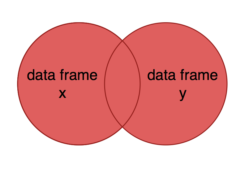
Full join
You might want a data frame that includes all data from both data sets, whether or not observations are missing in one or the other. This is analogous to including both circles in a Venn diagram.
Which observations would you expect to be included in the result of a full join using x = nutrients and y = carbon?
nutrients %>%
  full_join(y=carbon, by=c("Treatment", "Replicate"))
## Treatment Replicate Ammonium Nitrate Nitrite Carbon
## 1 1 1 8.2 1.7 0.4 42.5
## 2 1 2 6.9 3.6 1.5 NA
## 3 1 3 12.1 2.8 0.8 49.1
## 4 2 1 10.5 0.4 0.7 40.8
## 5 2 2 8.6 2.7 1.2 50.4
## 6 2 3 7.8 4.1 0.9 50.8
## 7 3 1 NA NA NA 45.6
## 8 3 2 NA NA NA 48.7
## 9 3 3 NA NA NA 43.5Challenge
- Create a data frame with data from all sites included in the data frames
genesandmetals, which we used for the left join challenges above.
Filtering joins
As demonstrated above, mutating joins compare observations from two data frames to determine which variables to add. In contrast, filtering joins keep only observations from the first data frame, and compare observations to a second data frame to determine which observations to keep. Filtering joins will only ever remove observations, and never add them.
There are two types of filtering joins:
- Semi joins (
semi_join) - keep all observations inxthat have a match iny - Anti joins (
anti_join) - keep all observations inxthat do not have a match iny
Semi join
Semi joins keep all observations in x that have a match in y. The Venn diagram depicting this join is the same as that for an inner_join.
The observations in the resulting data frame are also often the same as a inner_join. For example, compare the following:
nutrients %>%
  inner_join(y=carbon, by=c("Treatment", "Replicate"))
## Treatment Replicate Ammonium Nitrate Nitrite Carbon
## 1 1 1 8.2 1.7 0.4 42.5
## 2 1 3 12.1 2.8 0.8 49.1
## 3 2 1 10.5 0.4 0.7 40.8
## 4 2 2 8.6 2.7 1.2 50.4
## 5 2 3 7.8 4.1 0.9 50.8nutrients %>%
semi_join(y=carbon, by=c("Treatment", "Replicate"))## Treatment Replicate Ammonium Nitrate Nitrite
## 1 1 1 8.2 1.7 0.4
## 2 1 3 12.1 2.8 0.8
## 3 2 1 10.5 0.4 0.7
## 4 2 2 8.6 2.7 1.2
## 5 2 3 7.8 4.1 0.9Notice that the observations in both data frames are the same, but that the inner join adds the variable Carbon from the data frame carbon, whereas the semi join only uses the carbon data frame to determine which observations to keep.
Challenge
A semi join can be useful for determining the action of a
left_joinbefore calling it, i.e., to see what observations will have values that will be included, rather thanNA. Compare the output from following commands. Why are the data frames different if the data frames are joined usingby=c("Treatment")?nutrients %>% semi_join(y=carbon, by=c("Treatment", "Replicate")) nutrients %>% left_join(y=carbon, by=c("Treatment", "Replicate"))
Anti joins
Anti joins keep all observations in x that do not have a match in y. This might be useful if, for example, you have your main data in table x, and a second table that specifies data that you’d like to omit. Alternatively, this type of join might be part of a pipeline comparing an updated data frame to an older version to determine which observations are new.

An anti join can be used to determine which observations in x are missing data in y. Say we want to know which observations in nutrients are missing data in carbon. In this case, we could do the following:
  nutrients %>%
  anti_join(y=carbon, by=c("Treatment", "Replicate"))
## Treatment Replicate Ammonium Nitrate Nitrite
## 1 1 2 6.9 3.6 1.5Challenge
- What do you expect to see as a result of calling an anti join on
carbon, specifyingnutrientsas data framey? Describe this in words.